FinnishForestAI: R-Based LiDAR Forest Analysis

A reproducible workflow for Finnish airborne laser-scanning data

Abstract

This report documents the R implementation of FinnishForestAI, an open-source prototype for analysing airborne LiDAR point clouds for forest-structure applications. The workflow is designed around the National Land Survey of Finland (NLS) Laser scanning data 0.5 p product and combines point-cloud preprocessing, height normalization, forest metrics, canopy-height modelling, visualization, and a baseline machine-learning classifier.

The main objective is not to claim a production-ready forestry model. Instead, the project demonstrates how an AI/software-development background can be transferred to LiDAR, geospatial processing, and forestry-oriented analytical workflows using reproducible R code.

ImportantScope of this prototype

The bundled report renders by default with a synthetic point-cloud dataset so that the GitHub Pages build is lightweight and reproducible. When a real Finnish .las or .laz tile is supplied locally, the workflow switches to lidR-based terrain normalization and canopy rasterization. Results from the synthetic demonstration should not be interpreted as validation on real Finnish forests.

1. Motivation

Airborne laser scanning provides three-dimensional information about the ground and objects above it. The NLS describes each laser point using x, y, and z coordinates and identifies forest-resource information as one of the applications of laser-scanning data (National Land Survey of Finland 2026).

The practical question behind FinnishForestAI is:

Can open Finnish LiDAR data be transformed into a reproducible R workflow that derives useful forest-structure metrics and supports a baseline AI classification task?

The project focuses on five technical goals:

1. read and standardize point-cloud data;
2. estimate height above ground;
3. calculate interpretable forest-structure metrics;
4. generate a canopy-height representation; and
5. train a baseline machine-learning model from LiDAR point attributes.

2. Finnish LiDAR data

The target source is the NLS Laser scanning data 0.5 p product. According to the official product description, it is a three-dimensional point cloud thinned to approximately 0.5 points per square metre. The horizontal reference system is ETRS89 / TM35FIN (EPSG:3067), the vertical reference is N2000, and the distribution format is LAZ (National Land Survey of Finland 2026).

The NLS automatic classes that are especially useful for the current prototype are:

LAS class	Meaning	Height interpretation
2	Ground	Ground surface
3	Low vegetation	0.0–0.5 m above ground
4	Medium vegetation	0.5–2.0 m above ground
5	High vegetation	2.0–50.0 m above ground

These classifications are useful as a starting point, but they should not be treated as perfect ground truth. The NLS notes that the classifications are automatic and that users may filter or classify the data according to their own needs (National Land Survey of Finland 2026).

3. R technology stack

The R implementation uses the following packages:

• lidR — LiDAR/ALS point-cloud processing and canopy algorithms (Roussel et al. 2020);
• terra — raster handling and spatial outputs;
• ranger — efficient Random Forest modelling (Wright and Ziegler 2017);
• dplyr and readr — data manipulation and CSV input;
• ggplot2 — diagnostic and forest-profile visualization;
• jsonlite — machine-readable metric outputs.

For a local installation of the full real-LiDAR workflow:

Rscript r/install_packages.R

4. Workflow

flowchart TD
    A[Input: LAS / LAZ / CSV] --> B{Real LiDAR?}
    B -- Yes --> C[lidR readLAS]
    C --> D[Ground-based height normalization]
    D --> E[Normalized point cloud]
    B -- Demo CSV --> F[Portable 2% elevation baseline]
    F --> E
    E --> G[Forest height metrics]
    E --> H[Canopy height representation]
    E --> I[Classes 2-5 training data]
    I --> J[ranger Random Forest]
    J --> K[Baseline point classification]
    G --> L[CSV / JSON outputs]
    H --> M[Raster / figure outputs]

flowchart TD
    A[Input: LAS / LAZ / CSV] --> B{Real LiDAR?}
    B -- Yes --> C[lidR readLAS]
    C --> D[Ground-based height normalization]
    D --> E[Normalized point cloud]
    B -- Demo CSV --> F[Portable 2% elevation baseline]
    F --> E
    E --> G[Forest height metrics]
    E --> H[Canopy height representation]
    E --> I[Classes 2-5 training data]
    I --> J[ranger Random Forest]
    J --> K[Baseline point classification]
    G --> L[CSV / JSON outputs]
    H --> M[Raster / figure outputs]

The production R script implementing this workflow is r/forest_lidar_analysis.R.

5. Load the demonstration data

The GitHub report defaults to the bundled synthetic dataset. The code below mirrors the portable CSV branch of the R implementation.

is_las <- grepl("\\.(las|laz)$", input_file, ignore.case = TRUE)

if (is_las) {
  stop(
    "This GitHub-hosted report is configured for the portable CSV demo. ",
    "For a real LAS/LAZ run, use r/forest_lidar_analysis.R locally with lidR and terra installed."
  )
}

d <- read_csv(input_file, show_col_types = FALSE)
names(d) <- tolower(names(d))

stopifnot(all(c("x", "y", "z") %in% names(d)))

if (!"classification" %in% names(d)) d$classification <- 1
if (!"intensity" %in% names(d)) d$intensity <- 0
if (!"return_number" %in% names(d)) d$return_number <- 1
if (!"number_of_returns" %in% names(d)) d$number_of_returns <- 1

nrow(d)

[1] 61073

The bundled data are synthetic and exist only to exercise the workflow. They are not NLS observations.

6. Height normalization

For real LAS/LAZ input, the project uses NLS ground-class points and lidR::normalize_height(..., tin()). After normalization, the Z coordinate represents approximate height above terrain.

library(lidR)

las <- readLAS("data/raw/your_nls_tile.laz")
las_n <- normalize_height(las, tin())

For the portable synthetic CSV demonstration, no terrain surface is supplied. The project therefore uses the second percentile of Z as a simple baseline. This is deliberately a fallback for demonstration only, not a substitute for terrain normalization on real airborne LiDAR.

baseline <- as.numeric(quantile(d$z, 0.02, na.rm = TRUE))
d$height_agl <- pmax(d$z - baseline, 0)

baseline

[1] 90.75594

7. Forest-structure metrics

The first analytical output is a compact set of height and canopy metrics.

veg <- d$height_agl[d$height_agl > 0.5]
canopy <- d$height_agl[d$height_agl > 2]

metrics <- tibble(
  metric = c(
    "Points used",
    "Canopy cover > 2 m",
    "Mean vegetation height (m)",
    "Median vegetation height (m)",
    "P95 vegetation height (m)",
    "P95 canopy height (m)",
    "Maximum height above ground (m)"
  ),
  value = c(
    nrow(d),
    mean(d$height_agl > 2, na.rm = TRUE),
    mean(veg, na.rm = TRUE),
    quantile(veg, 0.50, na.rm = TRUE),
    quantile(veg, 0.95, na.rm = TRUE),
    quantile(canopy, 0.95, na.rm = TRUE),
    max(d$height_agl, na.rm = TRUE)
  )
)

kable(metrics, digits = 3, caption = "Forest-structure metrics for the bundled demonstration point cloud")

Forest-structure metrics for the bundled demonstration point cloud

metric	value
Points used	61073.000
Canopy cover > 2 m	0.792
Mean vegetation height (m)	8.160
Median vegetation height (m)	7.125
P95 vegetation height (m)	19.981
P95 canopy height (m)	20.594
Maximum height above ground (m)	30.520

The same values can be saved in machine-readable formats for downstream software:

write_csv(metrics, file.path(outdir, "quarto_metrics.csv"))
write_json(metrics, file.path(outdir, "quarto_metrics.json"), pretty = TRUE)

Interpretation

The P95 canopy height is often more robust than the absolute maximum because a single unusually high return can inflate the maximum. Canopy cover above 2 m is a simple structural indicator representing the fraction of analysed returns exceeding the high-vegetation threshold used by the NLS classes.

These metrics are useful descriptors, but they are not by themselves estimates of timber volume, biomass, basal area, or tree species. Those targets require suitable reference data and validation.

8. Height profile

set.seed(42)
plot_d <- d[sample(seq_len(nrow(d)), min(30000, nrow(d))), ]

ggplot(plot_d, aes(x = x, y = height_agl)) +
  geom_point(size = 0.25, alpha = 0.30) +
  labs(
    x = "Easting / synthetic X coordinate",
    y = "Height above ground (m)",
    title = "LiDAR height profile"
  ) +
  theme_minimal()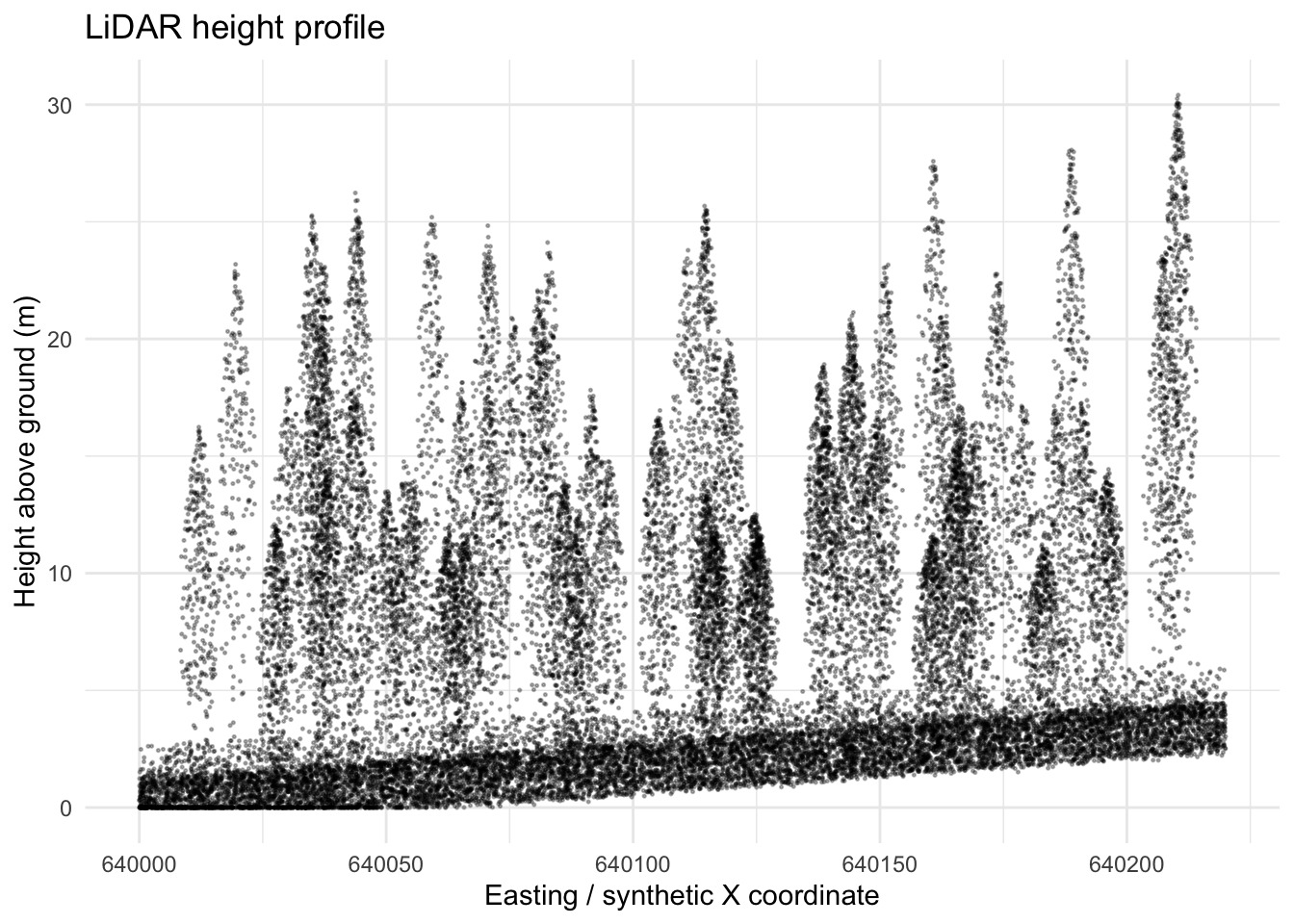

Sampled LiDAR height profile from the bundled synthetic forest point cloud.

The profile illustrates the key difference between ordinary 2D imagery and LiDAR: the analysis works with a vertical distribution of returns, not only pixel colour or intensity.

9. Canopy Height Model

For real point-cloud data, the R script uses lidR::rasterize_canopy() with a 2 m resolution and the point-to-raster (p2r) algorithm:

chm <- rasterize_canopy(las_n, res = 2, algorithm = p2r())
terra::writeRaster(chm, "outputs/r_run/canopy_height_model_R.tif", overwrite = TRUE)

For the portable synthetic demonstration, the report creates an equivalent 2 m maximum-height grid directly from the point table.

res <- 2
xmin <- min(d$x, na.rm = TRUE)
ymin <- min(d$y, na.rm = TRUE)

chm_demo <- d %>%
  mutate(
    gx = floor((x - xmin) / res) * res + xmin,
    gy = floor((y - ymin) / res) * res + ymin
  ) %>%
  group_by(gx, gy) %>%
  summarise(canopy_height_m = max(height_agl, na.rm = TRUE), .groups = "drop")

ggplot(chm_demo, aes(gx, gy, fill = canopy_height_m)) +
  geom_tile() +
  coord_equal() +
  labs(
    x = "X",
    y = "Y",
    fill = "Height (m)",
    title = "Canopy height representation"
  ) +
  theme_minimal()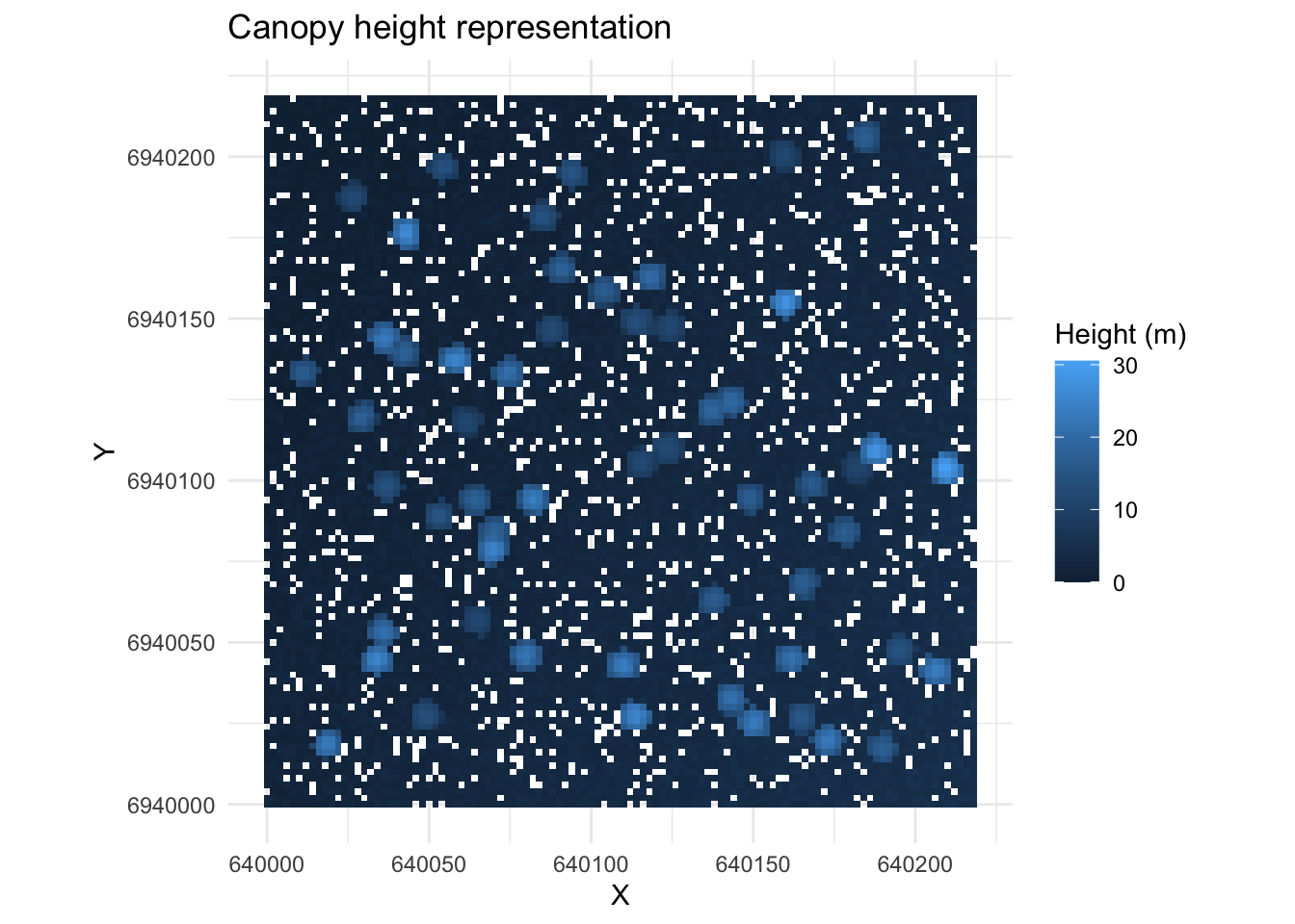

Portable 2 m canopy-height representation from the synthetic demonstration data.

A real Canopy Height Model is one of the most useful intermediate products for forestry-oriented LiDAR analysis because it converts normalized 3D returns into a spatial representation of upper-canopy height.

10. Baseline AI model

The R implementation uses NLS-style classes 2–5 as the baseline classification target and trains a Random Forest using four point-level predictors:

• height above ground;
• intensity;
• return number; and
• number of returns.

train <- d %>%
  filter(classification %in% c(2, 3, 4, 5)) %>%
  transmute(
    height_agl = height_agl,
    intensity = intensity,
    return_number = return_number,
    number_of_returns = number_of_returns,
    classification = factor(classification)
  )

set.seed(42)
if (nrow(train) > 100000) {
  train <- train[sample(seq_len(nrow(train)), 100000), ]
}

idx <- sample(seq_len(nrow(train)), floor(0.80 * nrow(train)))
train_set <- train[idx, ]
test_set <- train[-idx, ]

model <- ranger(
  classification ~ height_agl + intensity + return_number + number_of_returns,
  data = train_set,
  num.trees = 220,
  importance = "impurity"
)

pred <- predict(model, data = test_set)$predictions
cm <- table(Observed = test_set$classification, Predicted = pred)
accuracy <- sum(diag(cm)) / sum(cm)

accuracy

[1] 0.893246

kable(as.data.frame.matrix(cm), caption = "Held-out confusion matrix for the synthetic demonstration")

Held-out confusion matrix for the synthetic demonstration

	2	3	4	5
2	3553	0	21	3
3	226	31	209	3
4	542	36	654	120
5	49	0	95	6673

importance <- tibble(
  variable = names(model$variable.importance),
  importance = as.numeric(model$variable.importance)
) %>%
  arrange(desc(importance))

kable(importance, digits = 3, caption = "Random Forest variable importance")

Random Forest variable importance

variable	importance
height_agl	18094.661
number_of_returns	2829.962
intensity	2669.088
return_number	1151.755

WarningWhy this is only a baseline

The synthetic labels are intentionally related to height, so strong classification performance is expected and must not be presented as evidence of accuracy on real NLS data. In addition, the NLS classes themselves are automatic classifications rather than field-measured forestry labels. A serious forestry AI model should be evaluated using independent reference information.

11. What the current AI component demonstrates

The baseline model is technically useful because it demonstrates the complete engineering chain:

point cloud → preprocessing → feature construction → training data → Random Forest → prediction → evaluation → reusable model.

However, predicting the already available NLS vegetation classes is not the ultimate forestry objective. The more valuable next stage is to aggregate LiDAR-derived features to plots or grid cells and use independent forestry measurements as targets.

Possible future prediction tasks include:

• canopy-height classes;
• forest structural classes;
• vegetation density;
• stand-level attributes when appropriate reference labels are available;
• disturbance or change indicators using repeated acquisitions.

12. Running the R workflow on real Finnish LiDAR

Download a .laz tile from the NLS service and place it under data/raw/. Then run:

Rscript r/forest_lidar_analysis.R \
  data/raw/YOUR_FINNISH_TILE.laz \
  outputs/r_real_forest

The current script writes:

outputs/r_real_forest/
├── canopy_height_model_R.tif
├── forest_metrics_R.csv
├── forest_metrics_R.json
├── height_profile_R.png
├── vegetation_classifier_R.rds
└── variable_importance_R.json

The .rds file can be reloaded in R with:

model <- readRDS("outputs/r_real_forest/vegetation_classifier_R.rds")

13. Reproducibility and software design

The R implementation deliberately separates the reproducible analytical workflow from the optional user interface. The main analysis is contained in a command-line script, while r/app.R provides a small Shiny launcher.

This separation has several advantages:

• analysis can run without a graphical interface;
• jobs can be scripted or executed on HPC/cloud systems;
• input and output paths are explicit;
• outputs can be consumed by Python or other software;
• the workflow is easier to test, automate, and containerize.

The Python and R implementations therefore complement rather than replace each other. Python is useful for broader application engineering and ML integration, while R provides a mature ecosystem for statistical and forestry-oriented LiDAR analysis.

14. Limitations

The current R prototype has several important limitations:

1. No field-measured forestry targets are included. The model currently learns point classes rather than operational forest inventory variables.
2. The CSV fallback uses a crude terrain baseline. Real airborne LiDAR should use proper ground points and terrain normalization.
3. The current model is point-level. Many forestry decisions are made at tree, plot, raster-cell, or stand level.
4. Intensity can vary by acquisition conditions. It should not be assumed to be directly comparable across surveys without checking metadata and calibration.
5. No individual-tree segmentation is implemented yet. This would require additional algorithms and validation.
6. The 0.5 p product is relatively sparse. Some advanced single-tree tasks may benefit from denser point clouds where available.
7. Synthetic-demo accuracy is not real-world model validation. Independent Finnish forest reference data are required before making performance claims.

15. Next development phase

A stronger forestry AI version of FinnishForestAI should move from point-class prediction to a supervised forest-property modelling problem.

A proposed architecture is:

flowchart LR
    A[NLS LiDAR] --> C[Height normalization]
    C --> D[Grid / plot LiDAR metrics]
    B[Independent forest reference data] --> E[Spatial join]
    D --> E
    E --> F[Train / validation split]
    F --> G[ML model]
    G --> H[Forest-property predictions]
    H --> I[Map + uncertainty + validation]

flowchart LR
    A[NLS LiDAR] --> C[Height normalization]
    C --> D[Grid / plot LiDAR metrics]
    B[Independent forest reference data] --> E[Spatial join]
    D --> E
    E --> F[Train / validation split]
    F --> G[ML model]
    G --> H[Forest-property predictions]
    H --> I[Map + uncertainty + validation]

The independent reference layer could come from openly available Finnish forest-resource information where its variables and licensing are suitable for the intended experiment. This would allow the project to evaluate models against forestry-relevant targets rather than against the NLS automatic point classification.

16. GitHub Pages deployment

This repository includes a GitHub Actions workflow that renders the Quarto site from the bundled synthetic dataset and publishes _site/ to GitHub Pages.

Before publishing, replace USERNAME in _quarto.yml with your GitHub username and, if necessary, change the repository name in site-url and the GitHub navbar link.

Then enable Settings → Pages → Source → GitHub Actions in the repository. Every push to the default branch will rebuild the report.

For local rendering:

quarto preview

or:

quarto render

17. Conclusion

FinnishForestAI demonstrates a reproducible route from LiDAR point-cloud data to forestry-oriented analytical products using R. The current prototype includes data ingestion, height normalization, canopy and vegetation metrics, a canopy-height representation, machine-learning classification, model persistence, and diagnostic visualization.

The main value of the project is the integration of geospatial processing, LiDAR analysis, machine learning, and reproducible software engineering. The next scientific step is to connect LiDAR-derived features with independent Finnish forestry reference data and evaluate models for operational forest attributes using proper spatial validation.

References

National Land Survey of Finland. 2026. Laser Scanning Data 0.5 p. https://www.maanmittauslaitos.fi/en/maps-and-spatial-data/datasets-and-interfaces/product-descriptions/laser-scanning-data-05-p.

Roussel, Jean-Romain, David Auty, Nicholas C. Coops, et al. 2020. “lidR: An r Package for Analysis of Airborne Laser Scanning (ALS) Data.” Remote Sensing 12 (5): 730. https://doi.org/10.3390/rs12050730.

Wright, Marvin N., and Andreas Ziegler. 2017. “Ranger: A Fast Implementation of Random Forests for High Dimensional Data in c++ and r.” Journal of Statistical Software 77 (1): 1–17. https://doi.org/10.18637/jss.v077.i01.